IIR Filter Math and Calculations
IIR Filter Overview
An IIR (Infinite Impulse Response) filter is a digital filter that computes each output sample using both current and past input values as well as past output values. This feedback structure allows it to achieve sharp frequency responses with fewer coefficients than an FIR filter but can introduce stability and phase concerns.
General IIR Filter Equation
\[ y[n] = \sum_{k=0}^{M} b_k\,x[n-k] - \sum_{k=1}^{N} a_k\,y[n-k] \]
Second-Order (Biquad) IIR Filter Equation
\[ y[n] = b_0\,x[n] + b_1\,x[n-1] + b_2\,x[n-2] - a_1\,y[n-1] - a_2\,y[n-2] \]
Filter Flow Graphs
The most intuitive way to visualize an IIR filter is in Direct Form I. In this form, you can clearly see input samples being delayed (ie. \(x[n-1]\), \(x[n-2]\)), and being multiplied by a coefficient \(a_k\) and summed together. Likewise, output \(y[n]\) gets delayed (ie. \(y[n-1]\), \(y[n-2]\)), and scaled by \(b_k\) and summed together to find the current \(y[n]\).
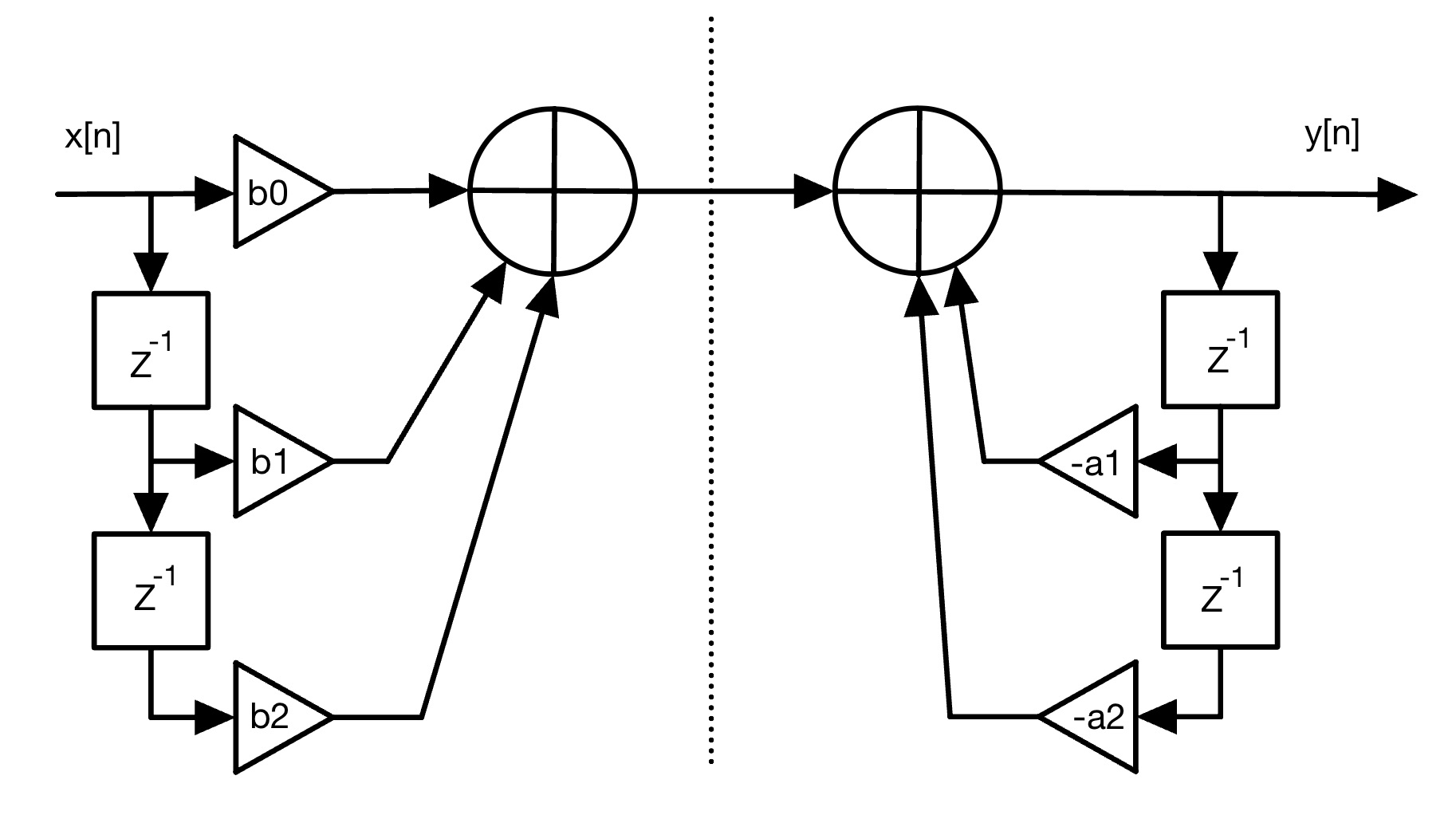
We can recognize that there are two independent linear systems on either side of the dashed line. A property of linear systems is that we can rearrange them. This leads us to the following intermediate form.
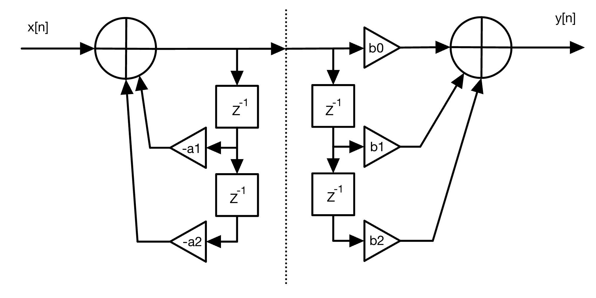
Looking at figure 2, the delay elements are in parallel with nothing in between them. This means that they are always the same values throughout the delay chain. We can reduce this redundancy by combining both sides to use the same delay elements.
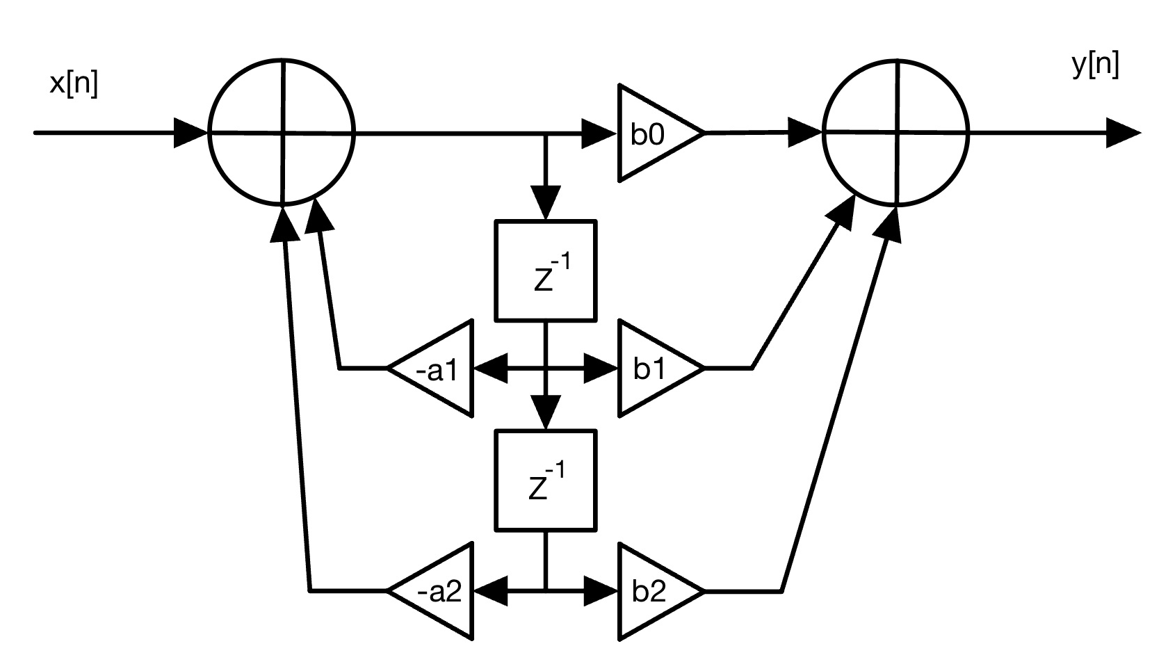
Figure 3 shows how the delay elements are combined to create the most compact implementation, known as Direct Form II. This structure is also the most memory-efficient, requiring only two stored values instead of four as in Direct Form I. Therefore, this is the form used for the IIR algorithm implemented on the FPGA.
Coefficient Calculations
Now that we understand the structure of the filter, we still need to calculate the \(a_k\) and \(b_k\) coefficients for our filters. Our 3-band EQ will consist of 3 cascading filters, one each for lows, mids, and highs. Each of these filters will consist of a second-order order IIR filter. Thus, the coefficients for each filter will be independent, being a fucntion of the potentiometer input of the corresponding band.
Our 3-band EQ uses three common second-order filter types. Each type has its own way of calculating the biquad coefficients \(a_k\) and \(b_k\).
Low Shelf Filter
A low shelf boosts or attenuates frequencies below a certain cutoff frequency (\(f_c\)). The coefficients are calculated from the desired cutoff, gain, and sampling rate:
\[ \begin{aligned} \omega &= 2 \pi \frac{f_c}{f_s} \\ A &= 10^{\text{gain}/40} \\ \alpha &= \frac{\sin(\omega)}{2} \sqrt{\frac{A+1}{A-1}} \\ b_0, b_1, b_2, a_0, a_1, a_2 &= \text{functions of } \omega, \alpha, A \end{aligned} \]
High Shelf Filter
A high shelf affects frequencies above a certain cutoff (\(f_c\)), either boosting or cutting them. The coefficient calculation is similar to the low shelf but reflects the change in frequency range:
\[ \begin{aligned} \omega &= 2 \pi \frac{f_c}{f_s} \\ A &= 10^{\text{gain}/40} \\ \alpha &= \frac{\sin(\omega)}{2} \sqrt{\frac{A+1}{A-1}} \\ b_0, b_1, b_2, a_0, a_1, a_2 &= \text{functions of } \omega, \alpha, A \end{aligned} \]
Peaking (Mid Cut / Boost) Filter
A peaking filter boosts or cuts a band of frequencies around a center frequency (\(f_c\)), defined by a Q-factor that sets the bandwidth:
\[ \begin{aligned} \omega &= 2 \pi \frac{f_c}{f_s} \\ \alpha &= \frac{\sin(\omega)}{2 Q} \\ A &= 10^{\text{gain}/40} \\ b_0, b_1, b_2, a_0, a_1, a_2 &= \text{functions of } \omega, \alpha, A \end{aligned} \]
Each of these formulas is then normalized by (\(a_0\)) to produce the final biquad coefficients (\(b_0, b_1, b_2, a_1, a_2\)) used in the FPGA implementation. The potentiometer for each band maps directly to the filter parameters (cutoff, gain, or Q), allowing real-time control.
Stability Considerations
IIR filters rely on feedback from past outputs, which means their stability must be carefully managed. For our 3-band EQ, stability is particularly important when using high gains or narrow Q-factors in the peaking (mid) filter, or extreme boost/cut in the low and high shelf filters.
A filter becomes unstable if the poles of its transfer function lie outside the unit circle in the z-plane. Practically, this can happen when: - Gain values are too large
- Q-factor is too high (causing a very narrow band with high resonance)
- Coefficient quantization on the FPGA introduces rounding errors
To ensure stable operation in our FPGA implementation, we: 1. Limit the maximum gain and Q values based on typical audio ranges.
2. Use Direct Form II to minimize memory usage but carefully handle scaling to avoid overflow.
3. Normalize all coefficients by (\(a_0\)) and use sufficient fixed-point precision for the coefficient representation.
By following these precautions, each band of the EQ remains stable across the full range of potentiometer settings, ensuring smooth and reliable real-time audio filtering.